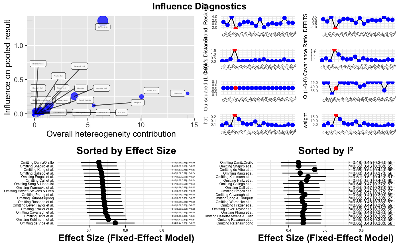
Conducts an influence analysis of meta-analysis results generated by meta functions
and produces influence diagnostic plots.
influence.analysis(x, random = FALSE, subplot.heights = c(30,18),
    subplot.widths = c(30,30), forest.lims = 'default',
    return.separate.plots = FALSE, text.scale = 1)
Arguments
| x | An object of class |
|---|---|
| random | Logical. Should the random-effects model be used to generate the influence diagnostics?
Uses the |
| subplot.heights | Concatenated array of two numerics. Specifies the heights of the
first (first number) and second (second number) row of the overall results plot generated by the function.
Default is |
| subplot.widths | Concatenated array of two numerics. Specifies the widths of the
first (first number) and second (second number) column of the overall results plot generated by the function.
Default is |
| forest.lims | Concatenated array of two numerics. Specifies the x-axis limits of the forest plots
generated by the function. Use |
| return.separate.plots | Logical. Should the influence plots be returned as seperate plots in lieue
of returning them in one overall plot? Additionally returns a dataframe |
| text.scale | Positive numeric. Scaling factor for the text geoms used in the plot. Values <1 shrink the
text, while values >1 increase the text size. Default is |
Value
If return.separate.plots is set to TRUE, a list object containing the
following objects is returned (if results are saved to a variable):
BaujatPlot: The Baujat plotInfluenceCharacteristics: The Viechtbauer-Cheung influence characteristics plotForestEffectSize: The forest plot sorted by effect sizeForestI2: The forest plot sorted by between-study heterogeneityData: Adata.framecontaining the data used for plotting.
Details
The function conducts an influence analysis using the "Leave-One-Out" paradigm internally and produces four diagnostic plots. These plots may be used to determine which study or effect size may have an excessive influence on the overall results of a meta-analysis and/or contribute substantially to the between-study heterogeneity in an analysis. This may be used for outlier detection and to test the robustness of the overall results found in an analysis. Four plots are produced, left to right, top to bottom:
Baujat Plot: Baujat et al. (2002) proposed a plot to evaluate heterogeneity patterns in a meta-analysis. The x-axis of the Baujat plot shows the overall heterogeneity contribution of each effect size while the y-axis shows the influence of each effect size on the pooled result. The
metainffunction is called internally to produce data used for plotting. Effect sizes or studies with high values on both the x and y-axis may be considered to be influential cases; effect sizes or studies with high heterogeneity contribution (x-axis) and low influence on the overall results can be outliers which might be deleted to reduce the amount of between-study heterogeneity.Influence Characteristics: Produces plots for several influence analysis diagnostics proposed by Viechtbauer & Cheung (2010). Data for plotting are generated by an internal call to
influence.rma.uni. Effect sizes/studies determined to be influential cases using the "rules of thumb" described in Viechtbauer & Cheung (2010) are plotted in red. For further details, see the documentation of theinfluence.rma.unifunction.Forest Plot for the Leave-One-Out Analysis, sorted by effect size: This forest plot displays the effect size and \(I^2\)-heterogeneity when omitting one of the \(k\) studies each time. The plot is sorted by effect size to determine which studies or effect sizes particularly affect the overall effect size. Results are generated by an internal call to
metainf.Forest Plot for the Leave-One-Out Analysis, sorted by I²: see above; results are sorted by \(I^2\) to determine the study for which exclusion results in the greatest reduction of heterogeneity.
References
Harrer, M., Cuijpers, P., Furukawa, T.A, & Ebert, D. D. (2019). Doing Meta-Analysis in R: A Hands-on Guide. DOI: 10.5281/zenodo.2551803. Chapter 6.3
DerSimonian R. & Laird N. (1986), Meta-analysis in clinical trials. Controlled Clinical Trials, 7, 177–188.
Viechtbauer, W., & Cheung, M. W.-L. (2010). Outlier and influence diagnostics for meta-analysis. Research Synthesis Methods, 1, 112–125.
See also
gosh.diagnostics, influence.rma.uni, metainf, baujat
Examples
# Load 'ThirdWave' data
data(ThirdWave)

# Create 'meta' meta-analysis object
meta = metagen(TE, seTE, studlab = paste(ThirdWave$Author), data=ThirdWave)

# Return seperate plots
influence.analysis(meta, subplot.heights = c(30,24), text.scale=0.5)#> [============================================================#> ===============] DONE
