Calculate the Surface Under the Cumulative Ranking score of from a network meta-analysis

This function calculates the SUCRA (Surface Under the Cumulative Ranking) score from a rank probability matrix or an object of class mtc.rank.probability generated by the rank.probability function.

Usage

sucra(x, lower.is.better = FALSE)

Arguments

x: An object of class mtc.rank.probability generated by the rank.probability function or a matrix/data.frame in which the rows correspond to the treatment, and columns to the probability of a specific treatment having this rank (see Details). Rownames of the matrix should contain the name of the specific treatment.
lower.is.better: Logical. Do lower (i.e., more negative) effect sizes mean that effects are higher? FALSE by default. Use the default when the provided matrix already contains the correct rank probability for each treatment, and values ought not to be inverted.

Details

The SUCRA score is a metric to evaluate which treatment in a network is likely to be the most efficacious in the context of network meta-analyses. The SUCRA score is calculated in the function using the formula described in Salanti, Ades and Ioannidis (2011): $$SUCRA_j = \frac{\sum_{b=1}^{a-1}cum_{jb}}{a-1}$$ Where $j$ is some treatment, $a$ are all competing treatments, $b$ are the $b = 1, 2, ..., a-1$ best treatments, and $cum$ represents the cumulative probability of a treatment being among the $b$ best treatments.

Other than an object of class mtc.rank.probability for argument x, the function can also be provided with a $m \times n$ matrix where $m$ are rows corresponding to each treatment in the network meta-analysis, and the $n$ columns correspond to each rank (1st, 2nd, etc.). Rank probabilities should be provided as a value from 0 to 1. Rownames of the matrix should correspond to the treatment names. Here is an example rank probability matrix for eight treatments:

.	[,1]	[,2]	[,3]	[,4]	[,5]	[,6]	[,7]	[,8]
CBT	0.000000	0.000000	0.000000	0.000000	0.000000	0.001275	0.087400	0.911325
IPT	0.000000	0.000000	0.000000	0.000000	0.000000	0.179400	0.745875	0.074725
PDT	0.000000	0.000000	0.000225	0.020300	0.978025	0.001450	0.000000	0.000000
PLA	0.002825	0.551175	0.262525	0.181550	0.001925	0.000000	0.000000	0.000000
PST	0.000000	0.000000	0.000000	0.000025	0.001450	0.817850	0.166725	0.013950
SUP	0.000000	0.216450	0.398700	0.383950	0.000900	0.000000	0.000000	0.000000
TAU	0.000375	0.229200	0.338525	0.414175	0.017700	0.000025	0.000000	0.000000
WLC	0.996800	0.003175	0.000025	0.000000	0.000000	0.000000	0.000000	0.000000

References

Harrer, M., Cuijpers, P., Furukawa, T.A, & Ebert, D. D. (2019). Doing Meta-Analysis in R: A Hands-on Guide. DOI: 10.5281/zenodo.2551803. Chapter 11.2.

Salanti, G., Ades, A. E. & Ioannidis, J.P.A. (2011). Graphical Methods and Numerical Summaries for Presenting Results from Multiple-Treatment Meta-Analysis: An Overview and Tutorial. Journal of Clinical Epidemiology, 64 (2): 163–71.

Author

Mathias Harrer & David Daniel Ebert

Examples

if (FALSE) {
# Example1 : conduct NMA using gemtc, calculate SUCRAs
suppressPackageStartupMessages(library(gemtc))
suppressPackageStartupMessages(library(igraph))
data("NetDataGemtc")

network = suppressWarnings(mtc.network(data.re = NetDataGemtc))

plot(network, layout = layout.fruchterman.reingold)

model = mtc.model(network, linearModel = "fixed",
                   n.chain = 4,
                   likelihood = "normal",
                   link = "identity")

mcmc = mtc.run(model, n.adapt = 5000, n.iter = 100000, thin = 10)

rp = rank.probability(mcmc)

sucra = sucra(rp, lower.is.better = TRUE)
sucra
plot(sucra)}



# Example 2: construct rank proabability matrix, then use sucra function
rp = rbind(CBT = c(0.000000, 0.000000, 0.000000, 0.000000, 0.000000, 0.001500, 0.088025, 0.910475),
           IPT = c(0.000000, 0.000000, 0.000000, 0.000000, 0.000000, 0.176975, 0.748300, 0.074725),
           PDT = c(0.000000, 0.000000, 0.000250, 0.021725, 0.976525, 0.001500, 0.000000, 0.000000),
           PLA = c(0.003350, 0.546075, 0.266125, 0.182125, 0.002325, 0.000000, 0.000000, 0.000000),
           PST = c(0.000000, 0.000000, 0.000000, 0.000000, 0.001500, 0.820025, 0.163675, 0.014800),
           SUP = c(0.000000, 0.217450, 0.403950, 0.378000, 0.000600, 0.000000, 0.000000, 0.000000),
           TAU = c(0.000225, 0.232900, 0.329675, 0.418150, 0.019050, 0.000000, 0.000000, 0.000000),
           WLC = c(0.996425, 0.003575, 0.000000, 0.000000, 0.000000, 0.000000, 0.000000, 0.000000))

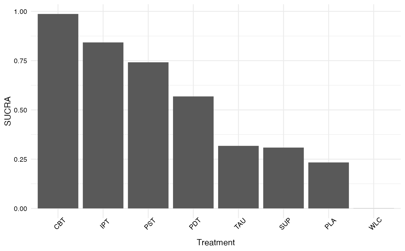
sucra(rp, lower.is.better = TRUE)
#>            SUCRA
#> CBT 0.9869964286
#> IPT 0.8425357143
#> PST 0.7416821429
#> PDT 0.5684678571
#> TAU 0.3175571429
#> SUP 0.3088214286
#> PLA 0.2334285714
#> WLC 0.0005107143
plot(sucra(rp, lower.is.better = TRUE))